![]()
![]()
![]()
Desirability functions are simple but useful tools for simultaneously optimizing several things at once. For each input, a translation function is used to map the input values between zero and one where zero is unacceptable and one is most desirable.
For example, Kuhn and Johnson (2019) use these functions during feature selection to help a genetic algorithm choose which predictors to include in a model that simultaneously improves performance and reduces the number of predictors.
The desirability2 package improves on the original desirability package by enabling in-line computations that can be used with dplyr pipelines.
Suppose a classification model with two tuning parameters
(penalty and mixture) and several performance
measures (multinomial log-loss, area under the precision-recall curve,
and the area under the ROC curve). For each tuning parameter, the
average number of features used in the model was also computed:
library(desirability2)
library(dplyr)
classification_results
#> # A tibble: 300 × 6
#>    mixture penalty mn_log_loss pr_auc roc_auc num_features
#>      <dbl>   <dbl>       <dbl>  <dbl>   <dbl>        <int>
#>  1       0  0.1          0.199  0.488   0.869          211
#>  2       0  0.0788       0.196  0.491   0.870          211
#>  3       0  0.0621       0.194  0.494   0.871          211
#>  4       0  0.0489       0.192  0.496   0.872          211
#>  5       0  0.0386       0.191  0.499   0.873          211
#>  6       0  0.0304       0.190  0.501   0.873          211
#>  7       0  0.0240       0.188  0.504   0.874          211
#>  8       0  0.0189       0.188  0.506   0.874          211
#>  9       0  0.0149       0.187  0.508   0.874          211
#> 10       0  0.0117       0.186  0.510   0.874          211
#> # ℹ 290 more rows
We might want to pick a model in a way that maximizes the area under the ROC curve with a minimum number of model terms. We know that the ROC measures is usually between 0.5 and 1.0. We can define a desirability function to maximize this value using:
d_max(roc_auc, low = 1/2, high = 1)For the number of terms, if we wanted to minimize this under the condition that there should be less than 100 features, a minimal desirability function can be appropriate:
d_min(num_features, low = 1, high = 100)We can add these as columns to the data using a mutate()
statement along with a call to the function that blends these values
using a geometric mean:
classification_results |>
  select(-mn_log_loss, -pr_auc) |>
  mutate(
    d_roc   = d_max(roc_auc, low = 1/2, high = 1),
    d_terms = d_min(num_features, low = 1, high = 50),
    d_both    = d_overall(d_roc, d_terms)
  ) |>
  # rank from most desirable to least:
  arrange(desc(d_both))
#> # A tibble: 300 × 7
#>    mixture penalty roc_auc num_features d_roc d_terms d_both
#>      <dbl>   <dbl>   <dbl>        <int> <dbl>   <dbl>  <dbl>
#>  1   1      0.0189   0.844            7 0.687   0.878  0.777
#>  2   1      0.0240   0.835            6 0.670   0.898  0.776
#>  3   0.889  0.0304   0.830            6 0.660   0.898  0.770
#>  4   0.778  0.0240   0.844            8 0.687   0.857  0.768
#>  5   0.778  0.0304   0.835            7 0.671   0.878  0.767
#>  6   0.889  0.0386   0.820            5 0.640   0.918  0.766
#>  7   0.889  0.0489   0.813            4 0.625   0.939  0.766
#>  8   0.667  0.0304   0.842            8 0.684   0.857  0.766
#>  9   0.778  0.0489   0.819            5 0.638   0.918  0.765
#> 10   0.778  0.0621   0.812            4 0.623   0.939  0.765
#> # ℹ 290 more rows
See ?inline_desirability for details on the individual
desirability functions.
We’ve also developed analogs to select_best()
and show_best()
that can be used to jointly optimize multiple metrics directly from an
object produced by the tune and finetune packages. We can load the
results for tune::tune_grid() for a pre-made binary
file:
library(tune)
library(ggplot2)

# Load the results from a cost-sensitive neural network:
load(system.file("example-data", "imbalance_example.rda", package = "desirability2"))

tuning_params <- .get_tune_parameter_names(imbalance_example)
tuning_params
#> [1] "hidden_units"  "penalty"       "activation"    "learn_rate"
#> [5] "stop_iter"     "class_weights"

metrics <- .get_tune_metric_names(imbalance_example)
metrics
#> [1] "kap"         "brier_class" "roc_auc"     "pr_auc"      "sensitivity"
#> [6] "specificity" "mn_log_loss" "mcc"
To demonstrate, we’ve fitted a neural network with several tuning
parameters, including one for class_weights. This parameter
makes the model cost-sensitive; if a weight of 2.0 is used, the
minority class in the training set has a 2-fold greater impact on the
estimation process.
For this example data set, increasing the class weight decreases specificity and increases sensitivity (at different rates). However, if we optimize on sensitivity, we are likely to get the worst specificity value.
nn_mtr <- collect_metrics(imbalance_example, type = "wide")
nn_mtr |>
  ggplot(aes(1 - specificity, sensitivity, col = class_weights)) +
  geom_point() +
  coord_obs_pred() +
  theme_bw() +
  theme(legend.position = "top")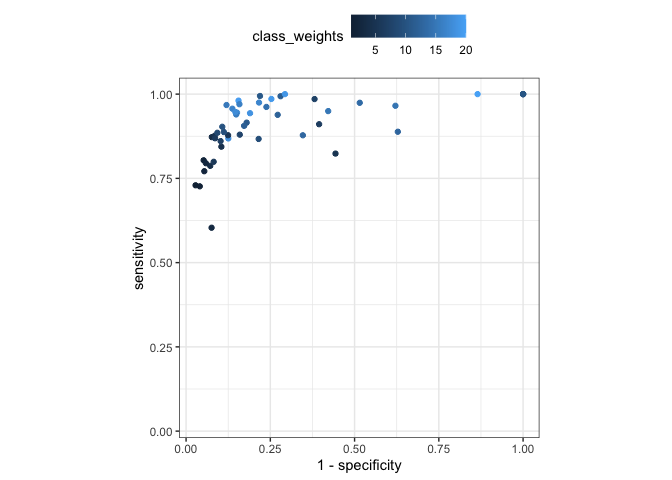
select_best(imbalance_example, metric = "sensitivity")
#> # A tibble: 1 × 7
#>   hidden_units penalty activation learn_rate stop_iter class_weights .config
#>          <int>   <dbl> <chr>           <dbl>     <dbl>         <dbl> <chr>
#> 1            5   0.391 tanh          0.00118      5.59          8.76 Preprocess…

select_best(imbalance_example, metric = "specificity")
#> # A tibble: 1 × 7
#>   hidden_units penalty activation learn_rate stop_iter class_weights .config
#>          <int>   <dbl> <chr>           <dbl>     <dbl>         <dbl> <chr>
#> 1           24 0.00910 relu           0.0164      1.92             1 Preprocess…

select_best(imbalance_example, metric = "brier_class")
#> # A tibble: 1 × 7
#>   hidden_units penalty activation learn_rate stop_iter class_weights .config
#>          <int>   <dbl> <chr>           <dbl>     <dbl>         <dbl> <chr>
#> 1           24 0.00910 relu           0.0164      1.92             1 Preprocess…
Also, we want to make sure our model is well calibrated so we also want to minimize the Brier score.
To do this, we can use different verbs: maximize(),
minimize(), target(), or
constrain() for any of the metrics or tuning
parameters. For example:
top_five <-
  imbalance_example |>
  show_best_desirability(
    # Put a little extra importance on the Brier scpre
    minimize(brier_class, scale = 2),
    maximize(sensitivity),
    constrain(specificity, low = 0.75, high = 1)
  )

# The resulting desirability functions and their overall mean
top_five |>
  select(starts_with(".d_"))
#> # A tibble: 5 × 4
#>   .d_min_brier_class .d_max_sensitivity .d_box_specificity .d_overall
#>                <dbl>              <dbl>              <dbl>      <dbl>
#> 1              0.842              0.918                  1      0.918
#> 2              0.770              0.951                  1      0.901
#> 3              0.808              0.891                  1      0.896
#> 4              0.763              0.924                  1      0.890
#> 5              0.806              0.866                  1      0.887

# The metric values (for most desirable to the fifth least desirable):
top_five |>
  select(all_of(metrics))
#> # A tibble: 5 × 8
#>     kap brier_class roc_auc pr_auc sensitivity specificity mn_log_loss   mcc
#>   <dbl>       <dbl>   <dbl>  <dbl>       <dbl>       <dbl>       <dbl> <dbl>
#> 1 0.703      0.0846   0.975  0.909       0.968       0.880       0.271 0.732
#> 2 0.643      0.102    0.968  0.877       0.981       0.844       0.323 0.684
#> 3 0.665      0.0925   0.972  0.901       0.957       0.863       0.298 0.699
#> 4 0.631      0.103    0.971  0.898       0.970       0.842       0.325 0.673
#> 5 0.642 0.0929 0.968 0.872 0.947 0.854 0.291 0.677Please note that the desirability2 project is released with a Contributor Code of Conduct. By contributing to this project, you agree to abide by its terms.
This project is released with a Contributor Code of Conduct. By contributing to this project, you agree to abide by its terms.
If you think you have encountered a bug, please submit an issue.
Either way, learn how to create and share a reprex (a minimal, reproducible example), to clearly communicate about your code.