The goal of fcirt is to estimate forced choice models using Bayesian method. Specifically, the Multi-Unidimensional Pairwise Preference (MUPP) model is estimated using the R package rstan that utilizes the Hamiltonian Monte Carlo sampling algorithm. Below are some important features of the fcirt package:
You can install fcirt from CRAN:
install.packages("fcirt")You can install the development version of fcirt from GitHub:
devtools::install_github("Naidantu/fcirt")This is a basic example which shows you how to prepare data, fit the model, extract and plot results:
library(fcirt)

## basic example code
## Step 1: Input data
# 1.1 Response data in wide format. If the first statement is preferred, the data should be coded as 1, otherwise it should be coded as 2.
fcirt.Data <- c(1,2,2,1,1,1,1,1,NA,1,2,1,1,2,1,1,2,2,NA,2,2,2,1,1,1,2,1,1,1,1,2,1,1,1,2,1,1,2,1,1)
fcirt.Data <- matrix(fcirt.Data,nrow = 10)
fcirt.Data
#>       [,1] [,2] [,3] [,4]
#>  [1,]    1    2    2    2
#>  [2,]    2    1    2    1
#>  [3,]    2    1    1    1
#>  [4,]    1    2    1    1
#>  [5,]    1    1    1    2
#>  [6,]    1    1    2    1
#>  [7,]    1    2    1    1
#>  [8,]    1    2    1    2
#>  [9,]   NA   NA    1    1
#> [10,]    1    2    1    1

# 1.2 A two-column data matrix: the first column is the statement number for statement s; the second column is the statement number for statement t.
pairmap <- c(1,3,5,7,2,4,6,8)
pairmap <- matrix(pairmap,ncol = 2)
pairmap
#>      [,1] [,2]
#> [1,]    1    2
#> [2,]    3    4
#> [3,]    5    6
#> [4,]    7    8

# 1.3 A column vector mapping each statement to each trait.
ind <- c(1,2,1,2,1,2,2,1)

# 1.4 A three-column matrix containing initial values for the three statement parameters (alpha, delta, tau) respectively. If using the direct MUPP estimation approach, 1 and -1 for alphas and taus are recommended and -1 or 1 for deltas are recommended depending on the signs of the statements. If using the two-step estimation approach, pre-estimated statement parameters are used as the initial values. The R package **bmggum** (Tu et al., 2021) can be used to estimate statement parameters for the two-step approach.
ParInits <- c(1, 1, 1, 1, 1, 1, 1, 1, 1, -1, 1, 1, 1, -1, 1, 1, -1, -1, -1, -1, -1, -1, -1, -1)
ParInits <- matrix(ParInits, ncol = 3)
ParInits
#>      [,1] [,2] [,3]
#> [1,]    1    1   -1
#> [2,]    1   -1   -1
#> [3,]    1    1   -1
#> [4,]    1    1   -1
#> [5,]    1    1   -1
#> [6,]    1   -1   -1
#> [7,]    1    1   -1
#> [8,]    1    1   -1

## Step 2: Fit the MUPP model
mod <- fcirt(fcirt.Data=fcirt.Data, pairmap=pairmap, ind=ind, ParInits=ParInits, iter=1000)

## Step 3: Extract the estimated results
# 3.1 Extract the theta estimates
theta <- extract(x=mod, pars='theta')
# Turn the theta estimates into p*trait matrix where p equals sample size and trait equals the number of latent traits
theta <- theta[,1]
# nrow=trait
theta <- matrix(theta, nrow=2)
theta <- t(theta)
# theta estimates in p*trait matrix format
theta
#>               [,1]         [,2]
#>  [1,] -0.008846518 -0.020839511
#>  [2,] -0.010909129  0.014170047
#>  [3,]  0.039271194 -0.029510418
#>  [4,]  0.053650150 -0.003515530
#>  [5,] -0.014835090 -0.038893088
#>  [6,] -0.029746453  0.003989843
#>  [7,]  0.046490462  0.007792688
#>  [8,]  0.027869493 -0.032391257
#>  [9,]  0.027951501 -0.011935207
#> [10,]  0.062773955 -0.012719476
# 3.2 Extract the tau estimates
tau <- extract(x=mod, pars='tau')
tau <- tau[,1]
tau
#>     tau[1]     tau[2]     tau[3]     tau[4]     tau[5]     tau[6]     tau[7]
#> -2.0540455 -0.9805878 -1.2825280 -1.4354192 -1.7621815 -1.0457171 -1.8182223
#>     tau[8]
#> -1.0445483
#3.3 Extract the estimates of the correlations among dimensions
cor <- extract(x=mod, pars='cor')

## Step 4: Plottings
# 4.1 Obtain the density plots for alpha
bayesplot(x=mod, pars='alpha', plot='density', inc_warmup=FALSE)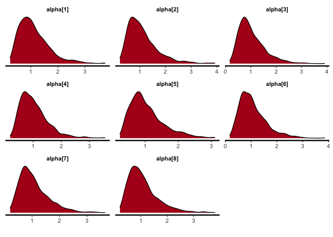
# 4.2 Obtain the trace plots for alpha
bayesplot(x=mod, pars='alpha', plot='trace', inc_warmup=FALSE)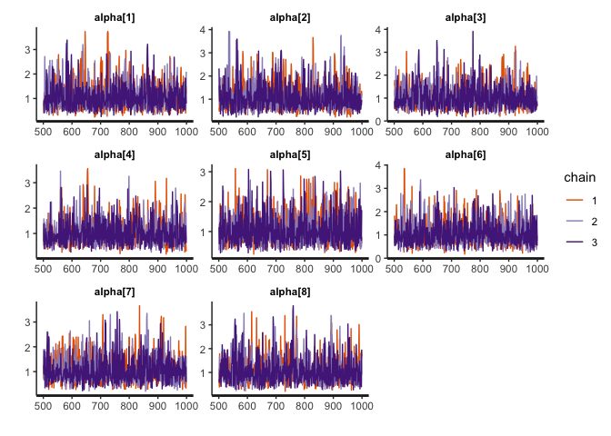
## Step 5: Item information
# 5.1 Obtain item information for item 1-3
OII <- information(x=mod, approach="direct", information="item", items=1:3)
OII
#> [1] 0.3915412 0.4035285 0.3920269
# 5.2 Obtain test information
OTI <- information(x=mod, approach="direct", information="test")
OTI
#> [1] 1.577941