| Type: | Package |
| Title: | Quantification of Lifecourse Fluidity |
| Version: | 2.0 |
| Date: | 2016-09-09 |
| Author: | Glenna Nightingale |
| Maintainer: | Glenna Nightingale <glenna.evans@gmail.com> |
| Description: | Provides in built datasets and three functions. These functions are mobility_index, nonStanTest and linkedLives. The mobility_index function facilitates the calculation of lifecourse fluidity, whilst the nonStanTest and the linkedLives functions allow the user to determine the probability that the observed sequence data was due to chance. The linkedLives function acknowledges the fact that some individuals may have identical sequences. The datasets available provide sequence data on marital status(maritalData) and mobility (mydata) for a selected group of individuals from the British Household Panel Study (BHPS). In addition, personal and house ID's for 100 individuals are provided in a third dataset (myHouseID) from the BHPS. |
| License: | GPL-2 | GPL-3 [expanded from: GPL] |
| Depends: | TraMineR,graphics |
| NeedsCompilation: | no |
| Packaged: | 2016-09-13 10:54:13 UTC; Glenna |
| Repository: | CRAN |
| Date/Publication: | 2016-09-13 14:40:35 |
lifecourse
Description
Quantifying lifecourse fluidity.
The mobility index function is provided together with in-built datasets. The mobility index function calculates the mobility index (number of distinct state episodes in a given sequence). The mobility index can be applied to different types of lifecourse channels apart from the migration channel. The output from this function gives an indication of the number of distinct state episodes within the lifecourse and hence the 'mobility' between state episodes. A state episode by definition would contain at least one state.
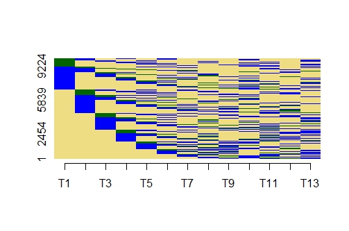
The difference in the average mobility index for three datasets is illustrated in the figures below. In the figures the lifecourse sequences for 10000 individuals (with their ID's on the y axis) over 13 years (denoted by T1 to T13 on the x axis) are shown. Each state can be either of four states (represented by yellow, blue, red and green blocks). In the first figure we note that there is a preponderance of yellow and blue blocks (which represent particular states). This dataset exhibits a high frequency of state episodes represented by either blue and yellow blocks. There are relatively few states represented by the green blocks and none represented by the red blocks. The average mobility index (over the 10000 sequences) is 6.52. This indicates that this dataset exhibits state episodes of high membership (recall that the lowest membership for a state episode is 1). The maximum value for the mobility index is 13 since the maximum number of years in the dataset is 13.
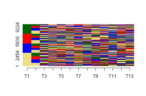
In the figure below, the states have been assigned randomly, and the average membership of the state episodes is much less than that in the previous dataset. Also all four of the possible states are evident in this dataset. For this dataset, the average mobility index is 10.54.
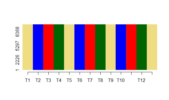
Finally, in the figure below each sequence contains states such that each successive state is different from that preceding it. In this case the mobility index for each sequence would be 13 and the average mobility index is 13. This indicates that this dataset exhibits high mobility between state episodes and the membership per episode is 1.
The in-built datasets are derived from the British Household Panel Survey data (BHPS). The data are derived from the BHPS indresp data files.
Details
| Package: | lifecourse |
| Type: | Package |
| Version: | 1.0 |
| Date: | 2016-03-18 |
| License: | GPL |
Author(s)
Glenna Nightingale <glenna.evans@gmail.com>
Examples
#---------------------------------------------------
# obtaining the in-built data derived from BHPS data.
#---------------------------------------------------
#data(mydata)
#bbc = mydata
#lbbc = length(mydata[,1])
#---------------------------------------------------
# plotting the sequences with the sequence states
# colour coded.
#--------------------------------------------------
#balphabet =c("non-mover","mover within gb")
# specifying the sequence alphabet.  For the BHPS mobility data we
# specify "non-mover" and "mover within gb"
#blabels = c("non-mover","mover within gb")
#bcodes =  c("non-mover","mover within gb")
#bseq = seqdef(bbc[,2:14], alphabet=balphabet,states = bcodes, labels = blabels)
# forming the dataset of sequences
#seqIplot(bseq,  sortv = "from.start",cex.legend=1.6,cex.main=3,cex.lab=1.5,cex = 2,
#         cpal=c("lightgoldenrod","blue"))
# plotting the sequences

#------------------------------------------
# calculating the mobility index
# for the observed sequences
#------------------------------------------
#bbcseq = bbc[,2:14]
# removing the first column which contains the ID for the persons involved.
#totalScore = score = 0
# calculating the mobility index for the observed sequences
#for(i in 1:length(bbcseq[,1])){
#  myseq = bbcseq[i,1:13]
#  score = (mobility_index(myseq,c("non-mover","mover within gb"),2))
#  totalScore = totalScore + score
#}
#totalScore
#testStatistic = totalScore/(13*lbbc)
# the length of the lifecourse = 13,
#the number of sequences = lbbc
#testStatistic

#-------------------------------------
# Running the non-standardization test
#-------------------------------------
#nll = nonStanTest(bbcseq,balphabet) # obtaining the null distribution
#hist(nll[[1]],main="Null distribution",xlab="Test statistsics",ylab="Frequency",col="grey")
# plotting the null distribution to compare with the observed test statistic.
#par(new=T)
#plot(density(nll[[1]],adjust=3),col="blue",axes=F,lwd=4,xlab="",ylab="",main="")
#abline(v=testStatistic,col="orange",lwd=4)
#nll[[2]]# Left Tailed test - pval
#nll[[3]]# Right Tailed test - pval
non-standardization test for lifecourses of linked lives
Description
The non-standardization test for lifecourses with linked lives. The simulations carried out for this test account for the fact that some individuals are more likely to have identical lifecourse trajectories. Acknowledgements: CPC St Andrews/Edinburgh.
Usage
linkedLives(currentData, sequenceUnits, lifecourseSequences)
Arguments
currentData |
Dataset containing a sequence of linking ID's (such as house ID's). |
sequenceUnits |
Vector containing the sequence alphabet. |
lifecourseSequences |
Dataset containing the sequences under invetigation. |
Author(s)
Glenna Nightingale
Examples
data(myHouseID)
data(mydata)
#------Exploring data---------
length(unique(myHouseID[,2]))
# number of unique individuals represented = 64
length((myHouseID[,2]))
# number of individuals in dataset = 100
length(myHouseID[,2])
# number of individuals represented = 100
hist(myHouseID[1:10,2],col="blue")
# plotting the first 10 house ID's
# Frequencies greater than 1 indicate individuals
# with the same house ID.
#--------------

#----- Running Function------------------
#B = linkedLives(myHouseID[,2:14],c("non-mover","mover within gb"),mydata[,2:14])
# the first column of the myHouseID and mydata
# datasets contain personal ID's
#----------------------------------------

#---- Plotting----------------------------
#hist(B[[1]],col="red",xlab="Simulated test statistics"
#,ylab="Frequency",main="Results of non-standardization test",
#cex.lab=1.5,xlim=c(range(B[[1]])[1],B[[4]]))
#abline(v=B[[4]],lwd=3,col="orange")
#B[[2]]# pval (Left tailed)
#B[[3]]# pval (Right tailed)
#B[[4]]# Empirical test statistic
#----------------------------------
Marital status sequences
Description
Each sequence contains the marital status for a given indivudal across 12 years. The sequence dataset is derived from data from the British Household Panel Survey.
Usage
data("maritalData")Format
A data frame with 4728 observations across 12 BHPS census waves.
Details
Each sequence represents a unique individual. The sequence alphabet is of length seven and the possible states are: "divorced", "have a dissoved civil partnership","in a civil partnership", "married", "never married", "separated", and "widowed".
Examples
library(TraMineR)
data(maritalData)

#-------------------------------------------
# Converting the data into a sequence object
#-------------------------------------------

#balphabet = c( "divorced" , "have a dissolved civil partnership" ,
#"in a civil partnership",  "married" ,
#"never married" ,"separated" ,"widowed" )

#blabels = c( "divorced" , "have a dissolved civil partnership" ,
#"in a civil partnership",  "married" ,
#"never married" ,"separated" ,"widowed" )

#bcodes = c( "divorced" , "have a dissolved civil partnership",
#"in a civil partnership",  "married" ,
#"never married" ,"separated" ,"widowed" )

#bseq = seqdef(maritalData, alphabet=balphabet,
#states = bcodes, labels = blabels)
# forming a sequence object


#-----------------------------
# Calculating the mobility index
# per sequence and storing
# the indices in an array
#-----------------------------
#lseq = length(bseq[,1])
#wseq = length(bseq[1,])
#sequence_summary = array(0,c(lseq,1))
#for(i in 1:lseq){
#sequence_summary[i] = mobility_index(bseq[i,],balphabet,7)
#}
#plot(hist(sequence_summary),xlim=c(1,7),col="red")

#---------------------------------------
# Generating subsets of the sequence data
#--------------------------------------
#seqIplot(bseq,  sortv = "from.start",cex.legend=1)
#mseq = bseq[which(bseq[,1]=="married"),] # sequences which start with the married state
#seqIplot(mseq,  sortv = "from.start",cex.legend=1)
#sseq = bseq[which(bseq[,1]=="never married"),] # sequences which start with the never married state
#seqIplot(sseq,  sortv = "from.start",cex.legend=1)

#------------------------------------
# Lifecourse destandardization
#------------------------------------
#object = summary(as.factor(sequence_summary))
#summarize = chisq.test(object,p = rep(1/length(object),9))
# assuming the "standard" probabilities is p = rep(1/length(object),9)
# alternative standard probabilities can be used.
#summary(maritalData)
mobility index
Description
Calculates the mobility index for a given sequence of states.
Arguments
sequence |
A given sequence of states |
alphabet |
Vector with sequence alphabet |
nalpha |
Length of sequence |
Details
The mobility index facilitates the calculation of each individual's mobility over the life course. This index is defined as the number of separate state clusters. A state cluster is defined as a bout of identical states (n>=1). Let A, B, and C denote the sequence alphabet for a given trajectory T = BABBAAAC. The mobility index assigned for T1 is 5 since there are 5 distinct state clusters: B, A, BB, AAA, and C. For a second trajectory, T2=BBBBBBBB, the mobility index is 1. The mobility index can be applied to different types of lifecourse data. The output from this function gives an indication of the number of state clusters within the lifecourse and hence the 'mobility' between states. The in-built datasets are derived from the British Household Panel Survey data (BHPS). The data are derived from the BHPS indresp data files.
Value
mobility index
Author(s)
Glenna Nightingale
Examples
#-----------------------------------------------------------------------
# Constructing 10000 sequences and calculating
#a test statistic (using the mobility index) from the resulting dataset.
#-----------------------------------------------------------------------

score = totalScore = 0
P = matrix("",nrow=10000,ncol=13)
myseq =  sample( LETTERS[c(1,4,5,7)], 13, prob=c(.25,.25,.25,.25), replace=TRUE )
# Each sequence contains four states.
#Examples of states are distinct geographical locations or marital status categories.
for(i in 1:10000){
myseq1 =  sample( myseq )
P[i,1:13] = myseq1
score = (mobility_index(myseq1,LETTERS[c(1,4,5,7)],13))
totalScore = totalScore + score
}
dataset_one_score = totalScore/(10000*13)
# test statistic =
#(sum of mobility index)/(total number of sequences * total number of years)
dataset_one_score
my house ID's
Description
House ID's for 100 individuals over 13 BHPS census waves. Each individual is labelled with a personal ID in the first column of the dataset.
Usage
data("myHouseID")Format
A data frame with 100 observations on the following 14 variables.
ida numeric vector
X1996a numeric vector
X1997a numeric vector
X1998a numeric vector
X1999a numeric vector
X2000a numeric vector
X2001a numeric vector
X2002a numeric vector
X2003a numeric vector
X2004a numeric vector
X2005a numeric vector
X2006a numeric vector
X2007a numeric vector
X2008a numeric vector
Details
The individuals represented in the dataset "mydata" are also represented in this dataset ("myHouseID").
Examples
data(myHouseID)
## maybe str(myHouseID) ; plot(myHouseID) ...
mydata
Description
A hundred mobility sequences representing 100 unique individuals. These data are derived from the British Household Panel Study (BHPS)dataset.
Usage
data("mydata")Format
A data frame with 100 observations on the following 14 variables.
ida numeric vector
X1996a factor with levels
mover within gbnon-moverX1997a factor with levels
mover within gbnon-moverX1998a factor with levels
mover within gbnon-moverX1999a factor with levels
mover within gbnon-moverX2000a factor with levels
mover within gbnon-moverX2001a factor with levels
mover within gbnon-moverX2002a factor with levels
mover within gbnon-moverX2003a factor with levels
mover within gbnon-moverX2004a factor with levels
mover within gbnon-moverX2005a factor with levels
mover within gbnon-moverX2006a factor with levels
mover within gbnon-moverX2007a factor with levels
mover within gbnon-moverX2008a factor with levels
mover within gbnon-mover
Examples
data(mydata)
## maybe str(mydata) ; plot(mydata) ...
non standardization test
Description
Allows the user to test a dataset of observed sequences to determine the probability that these sequences could have arisen due to chance. Acknowledgements: CPC St Andrews/Edinburgh.
Usage
nonStanTest(lifecourseSequences, sequenceUnits)
Arguments
lifecourseSequences |
A dataset (matrix form) consisting of sequences. |
sequenceUnits |
A vector containing the possible sequence states. |
Details
This is an approach to answering the question of whether or not the observed sequences for a given set of lifecourses could have arisen due to chance. This is achieved by comparing the observed sequences to a set of randomly simulated sequences .For each observed sequence A, there is a corresponding simulated sequence, B. B is constructed by assigning at random, an order to the observed states in A. The simulated sequences serve as a null distribution for the test.
Value
A p value (LeftTailed_pval) representing the probability that the observed test statistic (corresponding to the observed data) is greater than those obtained under the null hypothesis. A p value (RightTailed_pval) representing the probability that the observed test statistic (corresponding to the observed data) is less than those obtained under the null hypothesis.
The test statistics obtained under the null hypothesis are also provided.
Author(s)
Glenna Nightingale
Examples
data(mydata)
# obtaining the in-built data derived from BHPS data.
bbc = mydata
bbcseq = bbc[,2:14]
# removing the first column which contains the ID for the persons involved.
balphabet =c("non-mover","mover within gb")
#nll = nonStanTest(bbcseq,balphabet)
# obtaining the null distribution and p values