Index of /cran/web/packages/qatarcars/readme

	Name	Last modified	Size	Description
	Parent Directory		-
	man/	2025-10-16 14:00	-

qatarcars

Overview

Qatar Cars provides a more internationally-focused, modern cars-based demonstration dataset. It mirrors many of the columns in mtcars, but uses (1) non-US-centric makes and models, (2) 2025 prices, and (3) metric measurements, making it more appropriate for use as an example dataset outside the United States. It includes almost exactly the same variables as the mtcars dataset:

• origin (the country associated with the car brand)
• make (the brand of the car, such as Toyota or Land Rover)
• model (the specific type of car, such as Land Cruiser or Defender)
• length, width, and height (all in meters)
• trunk capacity (measured in liters)
• fuel economy (measured in liters per 100 km)
• performance (time in seconds to accelerate from 0 to 100km/h)
• mass in kilograms
• price in 2025 Qatari riyals
• type (the type of the car, such as coupe, sedan, or SUV)
• enginetype (electric, hybrid, or petrol)

The original data was compiled by Paul Musgrave in January 2025 and is mostly sourced from YallaMotors Qatar. See Paul’s writeup of the background and purpose of the data.

Formats

The Qatar Cars data is available in several different formats:

• This {qatarcars} R package. See below for complete details. Load like this:

  library(qatarcars)
  qatarcars

• Plain text CSV file. Use with any software.

• Stata .dta file. Load like this:

  use "qatarcars.dta"
  list in 1/6

• R .rds file. Load like this:

  df <- readRDS("qatarcars.rds")
  head(df)

• The QatarCars Python package. Install with pip install qatarcars, then load like this:

  from qatarcars import get_qatar_cars
  df = get_qatar_cars("pandas")  # or "polars"
  df.head()

Installation

The released version of {qatarcars} is available on CRAN:

install.packages("qatarcars")

You can also install the development version from GitHub:

# install.packages("remotes")
remotes::install_github("profmusgrave/qatarcars")

Usage

Load data

Similar to other data-only R packages like {gapminder} and {palmerpenguins}, load the data by running library(qatarcars):

library(qatarcars)

qatarcars
#> # A tibble: 99 × 15
#>    origin  make     model   length width height seating trunk economy horsepower
#>    <fct>   <fct>    <fct>    <dbl> <dbl>  <dbl>   <dbl> <dbl>   <dbl>      <dbl>
#>  1 Germany BMW      3 Seri…   4.71  1.83   1.44       5   480    11.8        184
#>  2 Germany BMW      3 Seri…   4.71  1.83   1.44       5    59     7.6        386
#>  3 Germany BMW      X1        4.50  1.84   1.64       5   505     6.6        313
#>  4 Germany Audi     RS Q8     5.01  1.69   2.00       5   605    12.1        600
#>  5 Germany Audi     RS3       4.54  1.85   1.41       5   321     8.7        400
#>  6 Germany Audi     A3        4.46  1.96   1.42       5   425     6.5        180
#>  7 Germany Mercedes Maybach   5.47  1.92   1.51       4   500    13.3        612
#>  8 Germany Mercedes G-Wagon   4.61  1.98   1.97       5   480    13.1        585
#>  9 Germany Mercedes EQS       5.22  1.93   1.51       5   610    NA          333
#> 10 Germany Mercedes GLA       4.41  1.83   1.61       5   435     5.6        163
#> # ℹ 89 more rows
#> # ℹ 5 more variables: price <dbl>, mass <dbl>, performance <dbl>, type <fct>,
#> #   enginetype <fct>

[!TIP]

If you have {tibble} installed (likely as part of the tidyverse), qatarcars will load as a tibble with nicer printing output; if you do not have {tibble} installed, the data will load as a standard data frame.

See ?qatarcars for data documentation within R.

Labels

Most columns in qatarcars are labeled:

attributes(qatarcars$economy)
#> $label
#> [1] "Fuel Economy (L/100km)"

These labels are visible in RStudio’s Viewer panel:

If you use {ggplot2} v4.0+, these variable labels will automatically appear in plot labels:

library(ggplot2)

ggplot(qatarcars, aes(x = economy)) + 
  geom_histogram(binwidth = 1, fill = "#8A1538", color = "white")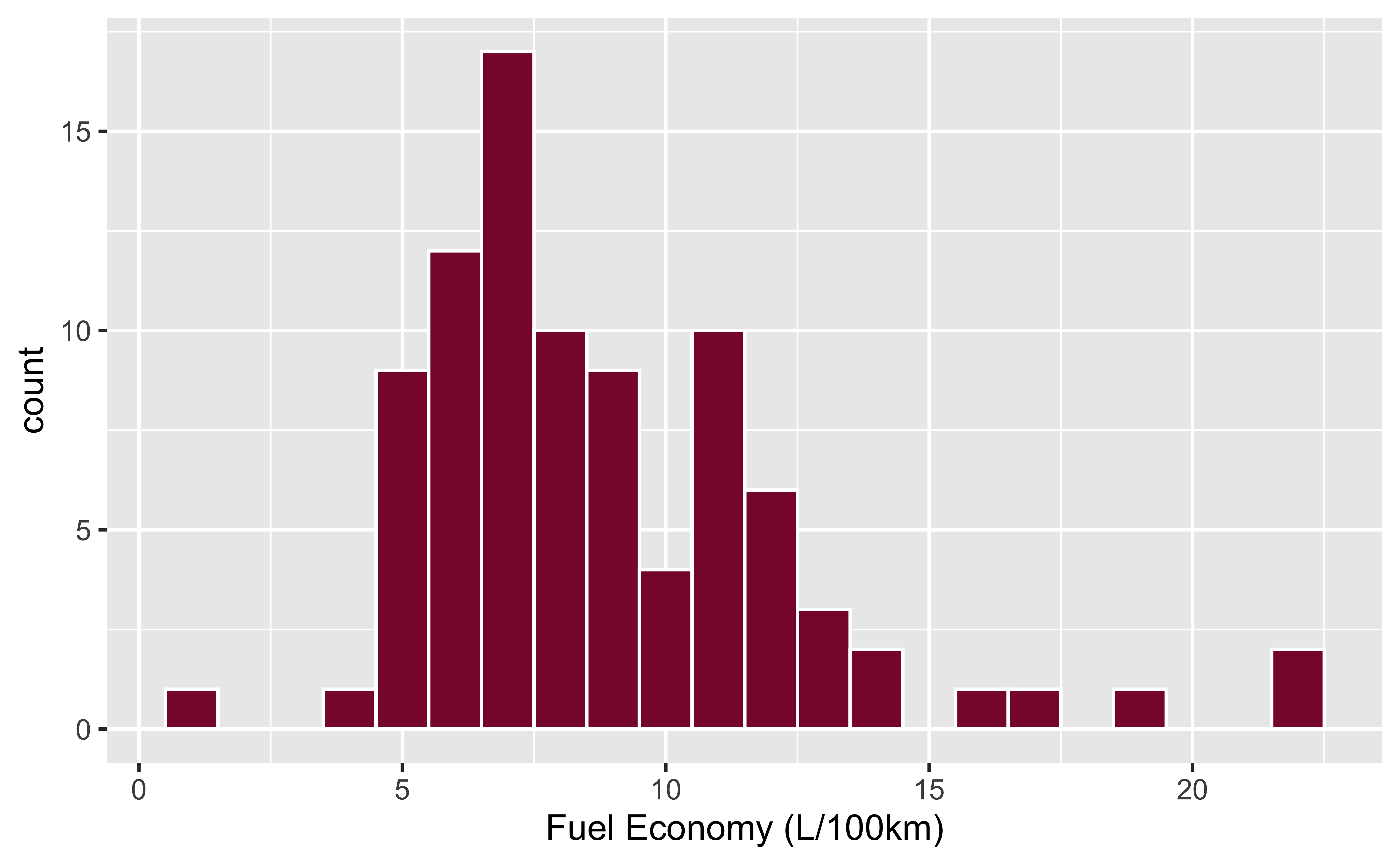

Examples

Fuel efficiency gets worse as cars get heavier:

ggplot(qatarcars, aes(x = mass, y = economy)) +
  geom_point() +
  geom_smooth(method = "lm") +
  scale_x_continuous(labels = scales::label_comma())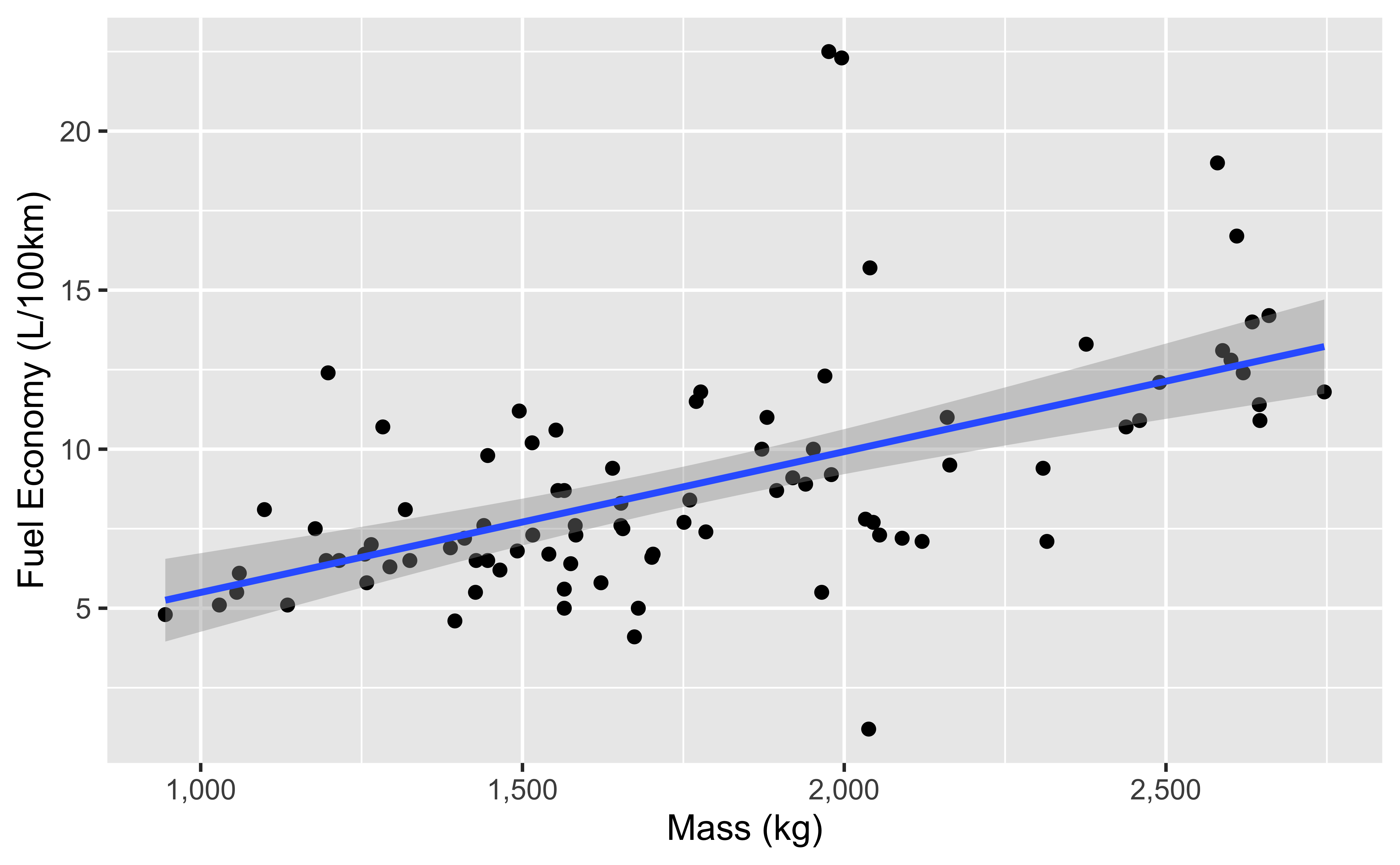

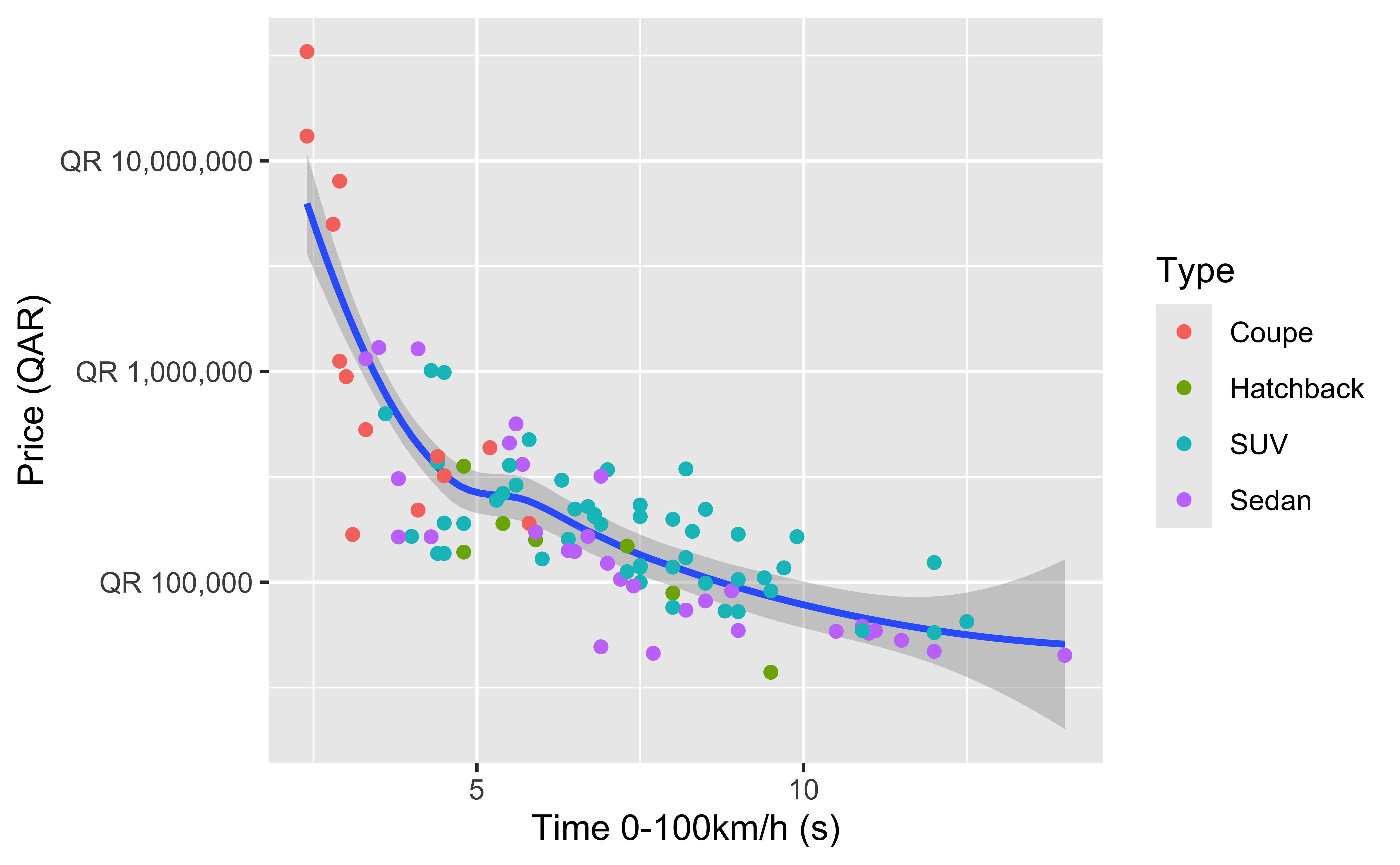
Some of these cars are really expensive, so logging the price is helpful:

ggplot(qatarcars, aes(x = performance, y = price)) +
  geom_smooth() +
  geom_point(aes(color = type)) +
  scale_y_log10(labels = scales::label_currency(prefix = "QR "))